 Looks like the Tiebout Sorting model — implemented as an app …
Tag: computational public policy
Visualizing Bank Failures ( 2008 – 2009 )
Three Takeaways
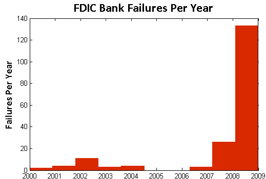
- Acceleration: There were four failures in the first six months of 2008, followed by another 22 failures in the next six months. By January of 2009, there were 21 failures in the first three months of the year, followed by 138 from April to last Friday.
- Magnitude: Failures in the past two years have cost the Depositors Insurance Fund an estimated $57B. The IndyMac failure of July 2008 accounted for $10B alone, followed by BankUnited at $4.9B and Guaranty Banks at $3B.
- Spatial Correlation: There is a significant amount of spatial correlation in California, Georgia, Florida, Texas, and Illinois. These states account for 77% of the total costs to the Depositors Insurance Fund. Furthermore, most of the losses in California and Georgia were concentrated highly around a few urban centers.
The Movie
The movie below shows the location of bank failures, beginning in 2008 and concluding with the three failed banks from Friday, December 11, 2009. Each green circle corresponds to a bank failure, and the size of each circle corresponds logarithmically to the FDIC’s estimated cost for the Depository Insurance Fund, as stated in the FDIC press releases. For failures with joint press releases, such as the 9 banks that failed on October 30th, the circles are sized in proportion to their relative total deposits.
Our visualization is similar to this one offered by the Wall Street Journal. For sizing the circles, the WSJ relied upon the value of assets at the time of failure. By contrast, our approach focuses upon the estimated impact to the Depositors Insurance Fund (DIF). In several instances, this alternative approach leads to a different qualitative result than the WSJ. For example, consider the case of Washington Mutual. While many have characterized Washington Mutual’s failure as the largest in history, according to the FDIC press release the failure did not actually lead to a draw upon Depositors Insurance Fund. By contrast, the FDIC estimated cost for the IndyMac Bank failure was substantial– the latest available estimate sets it at 10.7 billion.
Additional Background
As reported in a number of news outlets, Friday witnessed the failure of three more banks – Solutions Bank (Overland Park, KS), Valley Capital Bank (Mesa, AZ), and Republic Federal Bank (Miami, FL).
According to information obtained from the Federal Deposit Insurance Corporation (FDIC), there have been a total of 186 bank failures in the United States since 2000. Of these, 159 banks or roughly 85% have occurred in the past two years. The plot below displays the yearly failures since 2000. These 159 failures over the past two years have cost the Depositors Insurance Fund an estimated $57B.
In addition to the increase in the rate of bank failures, there has also been a substantial amount of spatial correlation between these failures. The table below shows the five states with the highest estimated total costs to the Depositors Insurance Fund since 2008. Together, these five states account for $44B of the total $57B in the past two years.
| State | Estimated Cost to Fund |
| California | $19.33B |
| Georgia | $9.29B |
| Florida | $6.77B |
| Texas | $4.56B |
| Illinois | $4.12B |
Cash for Clunkers – Visualization and Analysis
Cash for Clunkers: A Dynamic Map of the Cash Allowance Rebate Systems (CARS)
Some Background on the Car Allowance Rebate System (CARS)
From the official July 27, 2009 press release – “The National Highway Traffic Safety Administration (NHTSA) also released the final eligibility requirements to participate in the program. Under the CARS program, consumers receive a $3,500 or $4,500 discount from a car dealer when they trade in their old vehicle and purchase or lease a new, qualifying vehicle. In order to be eligible for the program, the trade-in passenger vehicle must: be manufactured less than 25 years before the date it is traded in; have a combined city/highway fuel economy of 18 miles per gallon or less; be in drivable condition; and be continuously insured and registered to the same owner for the full year before the trade-in. Transactions must be made between now [July 27, 2009] and November 1, 2009 or until the money runs out.”
On August 6, 2009, Congress extended the program adding $2 billion dollars to the program’s initial allocation. For those interested in background, feel free to read the CNN report on the program extension.
On August 13, 2009, the Secretary offered this press release noting “[T]he Department of Transportation today clarified that consumers who want to purchase new vehicles not yet on dealer lots can still be eligible for the CARS program. Dealers and consumers who have reached a valid purchase and sale agreement on a vehicle already in the production pipeline will be able to work with the manufacturer to receive the documentation needed to qualify for the program.”
On August 20, 2009, the Secretary announced the program would end on August 24, 2009 at 8pm EST. While this remained the deadline for sales, dealers were provided a small extension to file paperwork ( Noon on August 25, 2009). For those interested, all other press releases are available here.
The Cars.gov DataSet
The full data set is available for download here. From the Cars.gov website “these reports contain the transaction level information entered by participating dealers for the 677,081 CARS transactions that were paid or approved for payment as of Friday, October 16, 2009 at 3:00PM EDT for a total of $2,850,162,500. Please note that confidential financial or commercial information and consumer information protected under the DOT privacy policy has been redacted.” The official cars.gov website offers additional caveats on its note to analysts. One important thing to note, there is a statutory exemption which allowed transactions to occur pursuant to an amended rule after the August 24, 2009 termination date. Here is the relevant language of the amended rule:
“To qualify for the exception process, a dealer must have been prevented from submitting an application for reimbursement due to a hardship caused by the agency. Specifically, a dealer may request an exception if the dealer was locked out of the CARS system, contacted NHTSA for a password reset prior to the announced deadline, but did not receive a password reset. A dealer also may request an exception if its timely transaction was rejected by the CARS system due to a duplicate State identification number, trade-in vehicle VIN, or new vehicle VIN that was never used for a submitted CARS transaction, if the dealer contacted NHTSA prior to the announced deadline to resolve the issue but did not receive a resolution. Finally, a dealer may seek an exception if it was prevented from submitting a transaction by the announced deadline due to another hardship attributable to NHTSA’s action or inaction, upon submission of proof and justification satisfactory to the Administrator.”
For those who have downloaded the full set, the above passage explains why there exist transaction data which fall outside of the general CARS program window.
Dynamic Visualization of the Spatial Distribution of Sales
Each time step of the animation represents a day for which there exists data in the CARS official dataset. While the program officially started on July 27, 2009, the dataset contains both transactions undertaken during the pilot program as well as transactions undertaken pursuant the exemption process described above. Thus, the movie begins with the first unit of observation on July 1, 2009 and terminates with the final transaction on October 24, 2009. Similar to a flip book, the movie is generated by threading together each daily time slice.
The Size and Color of Each Circle
Each circle represents a zip code in which one or more participating dealerships is located. The radius of a given circle is function of the number of CARS related sales in a given zip code as of the date in question. In each day, the circle is colored if there is at least one sale in the current period while the circle is resized based upon the number of sales in the given period.
In the later days of the data window, particular those after official August 25 termination of the program, the daily sales are fairly negligible. However, as outlined in the dataset description above, each participating institution who qualified for the exemption was allowed to submit transactions beyond official program termination date. Notice the cumulative percentage of sales reach nearly all total sales by August 25th. Virtually all sales occur during the official July 27, 2009 – August 24, 2009 window. Thus, while these the stragglers caused certain circles to remain illuminated the size of circles is essentially fixed after August 24, 2009.
Some Things to Notice in the Visualization
In the lower left corner of the video, you will notice two charts. The chart on the left tracks the contribution to total sales for the given day. The chart on the right represent the cumulative percentage of sales to date under the program. Not surprisingly, most of the transactions under the CARS program take place between July 27, 2009 – August 24, 2009 time window.
Within this window, the daily sales feature a variety of interesting trends. During each Sunday of the program (i.e. August 2nd, August 9th, August 16th & August 23rd) sales were significantly diminished. Not surprisingly, the end of week and early weekend sales tend to be the strongest.
In the very early days of the program, there were a variety of media reports (e.g. here, here, here) highlighting the quickly dimishing resources under the program. Obviously, it is difficult to determine the underlying demand for the program. However, given the extent of the acceleration, it appears these reports contributed to the rapid depletion of the initial 1 billion dollars allocated under the program. A similar but less pronounced form of herding also accompanied the last days of the CARS program.
Electricity Market Simulations @ Argonne National Labs
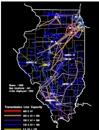
Given my involvement with the Gerald R. Ford School of Public Policy, many have justifiably asked me to describe how a computational simulation could assist in the crafting of public policy. The Electricity Market Simulations run at Argonne National Lab represent a nice example. These are high level models run over six decision levels and include features such as a simulated bid market. Argonne has used this model to help the State of Illinois as well as several European countries regulate their markets for electricity.
A Statistical Mechanics Take on No Child Left Behind — Flow and Diffusion of High-Stakes Test Scores [From PNAS]
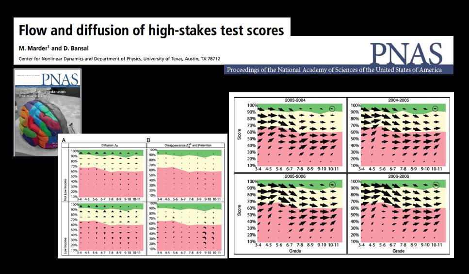
The October 13th Edition of the Proceedings of the National Academy of Science features a very interesting article by Michael Marder and Dhruv Bansal from the University of Texas.
From the article … “Texas began testing almost every student in almost every public school in grades 3-11 in 2003 with the Texas Assessment of Knowledge and Skills (TAKS). Every other state in the United States administers similar tests and gathers similar data, either because of its own testing history, or because of the Elementary and Secondary Education Act of 2001 (No Child Left Behind, or NCLB). Texas mathematics scores for the years 2003 through 2007 comprise a data set involving more than 17 million examinations of over 4.6 million distinct students. Here we borrow techniques from statistical mechanics developed to describe particle flows with convection and diffusion and apply them to these mathematics scores. The methods we use to display data are motivated by the desire to let the numbers speak for themselves with minimal filtering by expectations or theories.
The most similar previous work describes schools using Markov models. “Demographic accounting” predicts changes in the distribution of a population over time using Markov models and has been used to try to predict student enrollment year to year, likely graduation times for students, and the production of and demand for teachers. We obtain a more detailed description of students based on large quantities of testing data that are just starting to become available. Working in a space of score and time we pursue approximations that lead from general Markov models to Fokker–Planck equations, and obtain the advantages in physical interpretation that follow from the ideas of convection and diffusion.”
The Dynamics of Deterrence – New Article in PNAS
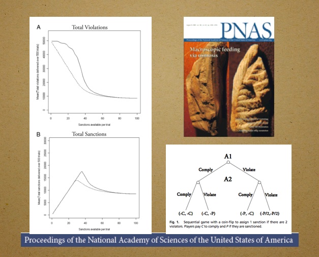
The latest edition of the Proceedings of the National Academy of Science (PNAS) features The Dynamics of Deterrence by Mark Kleiman & Beau Kilmer. Here is the abstract: “Because punishment is scarce, costly, and painful, optimal enforcement strategies will minimize the amount of actual punishment required to effectuate deterrence. If potential offenders are sufficiently deterrable, increasing the conditional probability of punishment (given violation) can reduce the amount of punishment actually inflicted, by “tipping” a situation from its high-violation equilibrium to its low-violation equilibrium. Compared to random or “equal opportunity” enforcement, dynamically concentrated sanctions can reduce the punishment level necessary to tip the system, especially if preceded by warnings. Game theory and some simple and robust Monte Carlo simulations demonstrate these results, which, in addition to their potential for reducing crime and incarceration, may have implications for both management and regulation.”
Visualizing 26 U.S.C ___ : At the “Section Depth”
Title 26 of the United States Code is likely on the mind of many as we move toward April 15th. As a part of a project with Lilian V. Faulhaber (Climenko Fellow from HLS), we have become interested in the architecture of 26 U.S.C. ___.
As we define it, a “section depth” representation for 26 U.S.C. 501(c)(3) represents a traversal to the level of Sec. 501. While a “full depth” representation would include a mapping beyond Sec. 501 to its (c) and (3) subcomponents. In our previous post highlighting 11 U.S.C. __ (the Bankruptcy Code), we presented a traversable “full depth” representation for its structure.
Considering all 50 titles of the United States Code, 26 U.S.C. __ is among the largest of the titles in its architectural size and depth. In fact, given its size, it is not possible for us to render for public consumption, a labeled, “full depth” and zoomable representation for all of 26 U.S.C. ___.
Above we provide a “section depth” representation for 26 U.S.C __ where the terminal nodes are sections such Sec. 1031. You will notice that this section depth representation is roughly the size of the full depth representation we provide for 11 U.S.C. ___. We have colored in Green the primary Income Tax Sections under 26. The documentation is similar to that for 11 U.S.C. ___ thus please refer to this post for additional information. However, for traversal purposes, it is important to remember to start in the middle at the “26 U.S.C.” and follow the branch of the graph out to a leaf node.
We believe the comparative consideration of the architecture for these titles offers a rough first cut on questions of code magnitude and complexity. Although it is a first order approximation and we do believe layering in the relevant administrative regulations and jurisprudence to these sections would represent an improvement on the question, it still bears asking whether it would drastically alter the macro state of affairs. That is an empirical question and only time will tell.
Google for Government? Broad Representations of Large N DataSets
In our previous post, a post which has generated tremendous interest from a variety of sources, we demonstrated how applying the tools of network science can provide a broad representation for thousands of lines of information. Throughout the 2008 Presidential Campaign then Senator Obama consistently discussed his Google for Government initiative.
From the Obama for America Website:
Google for Government: Americans have the right to know how their tax dollars are spent, but that information has been hidden from public view for too long. That’s why Barack Obama and Senator Tom Coburn (R-OK) passed a law to create a Google-like search engine to allow regular people to approximately track federal grants, contracts, earmarks, and loans online.
We agree with both President Obama and Senator Coburn that universal accessibility of such information is worthwhile goal. However, we believe this is only a first step.
In a deep sense, our prior post is designed to serve as a demonstration project. We are just two graduate students working on a shoestring budget. With the resources of the federal government, however, it would certainly be possible to create a series of simple interfaces designed to broadly represent of large amounts of information. While these interfaces should rely upon the best available analytical methods, such methods could probably be built-in behind the scenes. At a minimum, government agencies should follow the suggestion of David G. Robinson and his co-authors who argue the federal government “should require that federal websites themselves use the same open systems for accessing the underlying data as they make available to the public at large.”
Anyway, will be back on Monday providing more thoughts on our initial representation of the 110th Congress. In addition, we hope to highlight other work in the growing field of Computational Legal Studies. Have a good rest of the weekend!

