Month: October 2009
Electricity Market Simulations @ Argonne National Labs
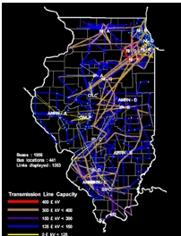
Given my involvement with the Gerald R. Ford School of Public Policy, many have justifiably asked me to describe how a computational simulation could assist in the crafting of public policy. The Electricity Market Simulations run at Argonne National Lab represent a nice example. These are high level models run over six decision levels and include features such as a simulated bid market. Argonne has used this model to help the State of Illinois as well as several European countries regulate their markets for electricity.
The Structure of the United States Code [w/ Zoomorama] [Repost]
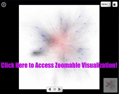
Formally organized into 50 titles, the United States Code is the repository for federal statutory law. While each of the 50 titles define a particular substantive domain, the structure within and across titles can be represented as a graph/network. In a series of prior posts, we offered visualizations at various “depths” for a number of well know U.S.C. titles. Click here and click Here for our two separate visualizations of the Tax Code (Title 26). Click here for our visualization of the Bankruptcy Code (Title 11). Click here for our visualization of Copyright (Title 17). While our prior efforts were devoted to displaying the structure of a given title of the US Code, the visualization above offers a complete view of the structure of the entire United States Code (Titles 1-50).
Using Zoomorama, each title is labeled with its respective number. The small black dots are “vertices” representing all sections in the aggregate US Code (~37,500 total sections). Given the size of the total undertaking, in the visual above, every title is represented to the “section level.” As we described in earlier posts, a “section level” representation halts at the section and thus does not represent any of subsection depth. For example, all sections under 26 U.S.C. § 501 including the well known § 501 (c) (3) are reattributed upward to their parent section.
There are two sources of structure within the United States Code. The explicitly defined structure / linkage / dependancy derives from the sections contained under a given title. The more nuanced version of structure is obtained from references or definitions contained within particular sections. This class of connections not only link sections within a given title but also connection sections across titles. Within this above visual, we represent these important cross-title references by coloring them red.
Taken together, this full graph of the Untied States Code is quite large {i.e. directed graph (|V| = 37500, |E| = 197749)}. There exist 37,500 total sections distributed across the 50 Titles. However, these sections are not distributed in a uniform manner. For example, components such as Title 1 feature very few sections while Titles such as 26 and 42 contain many sections. The number of edges far outstrips the number of vertices with a total 197,000+ edges in the graph.
We are currently writing the paper on this subject … so please consider this the trailer. Above we offer the same visual of the United States Code (Titles 1-50) which we previously offered here … this time we are using Zoomorama. Zoomorama is an alternative to Seadragon which we believe might perform better on certain machine configurations.
If you click on the image above you should be taken straight to the full page image. From there you should be click to zoom in and then read the titles … For those unfamiliar, please click here for the Zoomorama Instructions!
United States Court of Appeals & Parallel Tag Clouds from IBM Research
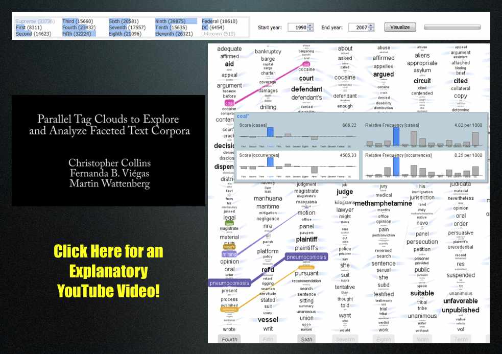
Download the paper: Collins, Christopher; Viégas, Fernanda B.; Wattenberg, Martin. Parallel Tag Clouds to Explore Faceted Text Corpora To appear in Proceedings of the IEEE Symposium on Visual Analytics Science and Technology (VAST), October, 2009. [Note: The Paper is 24.5 MB]
Here is the abstract: Do court cases differ from place to place? What kind of picture do we get by looking at a country’s collection of law cases? We introduce Parallel Tag Clouds: a new way to visualize differences amongst facets of very large metadata-rich text corpora. We have pointed Parallel Tag Clouds at a collection of over 600,000 US Circuit Court decisions spanning a period of 50 years and have discovered regional as well as linguistic differences between courts. The visualization technique combines graphical elements from parallel coordinates and traditional tag clouds to provide rich overviews of a document collection while acting as an entry point for exploration of individual texts. We augment basic parallel tag clouds with a details-in-context display and an option to visualize changes over a second facet of the data, such as time. We also address text mining challenges such as selecting the best words to visualize, and how to do so in reasonable time periods to maintain interactivity.
Programming Dynamic Models in Python: Coding Efficient Dynamic Models
 In the next few tutorials, we’re going to transition to exploring how to model dynamics on a network.
The first tutorial was a bit of a blockbuster length-wise because there was a lot of ground to cover to get the basic model up and running. Moving forward, we’ll be able to go a bit more incrementally, adding elements to the basic model as we go. If you don’t feel comfortable with the original, go back and take a look at it and make sure that it makes sense to you before moving on.
We’re first going to deal with some of the efficiency issues in the first model. After this, we’ll make some basic changes to the architecture of the SIR program that makes it more amenable to contact patterns on a social network.
Finally, we’ll show you how to how to take the output of your epidemic model and generate animations like this one:
Blue nodes are exposed but uninfected, red nodes are infectious, and yellow ones have recovered.
The movie is a bit of a carrot to get you through the less flashy, but, I promise, important and actually interesting nuts and bolts of putting these kinds of models together.
This tutorial is going to cover the last two big things that we need to tackle before we get to the model of an outbreak on a network. So, here we go!
New Concepts
1. Arbitrarily Distributed Infectious Periods
First, we’re going to deal with the duration of the infectious period. The assumption of an exponentially distributed infectious period is unnecessarily restrictive for a general model of diffusion, and the way the original code goes about recovering individuals – drawing a random number on every step for every infectious individual – should strike you as both inelegant and computationally inefficient, particularly when the rate of recovery is slow and there are many infectious individuals.
In order to deal with this, we’re going to introduce two new tools. The first is the scipy.stats toolkit and the second is a neat (and very easy to use) data structure called a heap.
A heap is in very many ways what it sounds like: imagine a pile of trash in a landfill; the tires and rusting washing machines are on the bottom, while the pop cans and grocery store receipts are closer to the top.
As a programming tool, a heap is useful because it always keeps the smallest (or largest, depending on your preference) item at the top of the list. It also allows for linear-time insertion and removal of objects. This means that the time it takes to execute an action grows proportionally to the size of the list, so if it has N items, it takes N*C steps (where C is a constant) to process the list, and if it has 2*N items, it takes 2*N*C steps. Other ways of sorting could take N^2 or worse steps to do the same.
In our outbreak model, the top item on the heap is always going to be the time at which the next individual recovers. By doing this, we can avoid the loop in the first tutorial (and replicated in one implementation here) that checks whether each infectious individual is going to recover on each step.
Looping over everyone is the most intuitive way to check if they’re going to recover, but it’s very inefficient, especially when infectious periods are long and the population is large. It’s also problematic from a theoretical perspective, because it chains us to exponentially distributed recovery periods.
Exponentially distributed infectious periods make analytic sense for a deterministic model, but your disease or *insert diffusible here* may have a constant or normally distributed ‘infectious’ period.
By using a heap-based implementation, as you will see, we can use arbitrary recovery periods, and Python’s implementation of the heap is very straightforward – just a small twist on the usual list using the heapq module.
2. Object Oriented Programming
One of Python’s strengths is that it supports a style of programming that mixes the best of object-oriented programming (OOP) and procedural or imperative programming.
We won’t go too deep into the details of OOP here, but the real strength of OOP implementations are that they allow code to be easily re-used in other programs (Python’s all-powerful ‘import‘ statement really makes this true) and also forces some structure on what functions have access to what variables, etc.
Click Below to Review the Implementation and Commented Code!
Continue reading “Programming Dynamic Models in Python: Coding Efficient Dynamic Models”
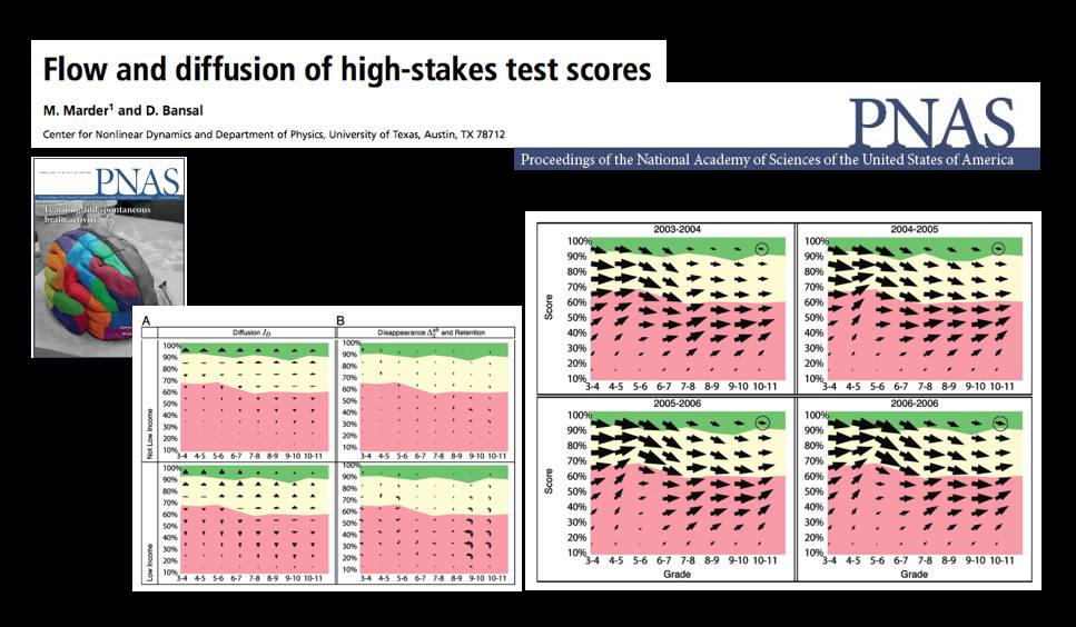
A Statistical Mechanics Take on No Child Left Behind — Flow and Diffusion of High-Stakes Test Scores [From PNAS]
The October 13th Edition of the Proceedings of the National Academy of Science features a very interesting article by Michael Marder and Dhruv Bansal from the University of Texas.
From the article … “Texas began testing almost every student in almost every public school in grades 3-11 in 2003 with the Texas Assessment of Knowledge and Skills (TAKS). Every other state in the United States administers similar tests and gathers similar data, either because of its own testing history, or because of the Elementary and Secondary Education Act of 2001 (No Child Left Behind, or NCLB). Texas mathematics scores for the years 2003 through 2007 comprise a data set involving more than 17 million examinations of over 4.6 million distinct students. Here we borrow techniques from statistical mechanics developed to describe particle flows with convection and diffusion and apply them to these mathematics scores. The methods we use to display data are motivated by the desire to let the numbers speak for themselves with minimal filtering by expectations or theories.
The most similar previous work describes schools using Markov models. “Demographic accounting” predicts changes in the distribution of a population over time using Markov models and has been used to try to predict student enrollment year to year, likely graduation times for students, and the production of and demand for teachers. We obtain a more detailed description of students based on large quantities of testing data that are just starting to become available. Working in a space of score and time we pursue approximations that lead from general Markov models to Fokker–Planck equations, and obtain the advantages in physical interpretation that follow from the ideas of convection and diffusion.”
Reading List – Law as a Complex System {Updated Version 10.16.09}
Several months ago, I put together this syllabus for use in a hypothetical seminar course entitled Law as a Complex System. I hoped to revise this reading list / syllabus and have now done so …. While this revised version might contain more content than would be practical for the typical 2-3 credit seminar, I do believe it is far more reasonable than Version 1.0. For anyone who is interested in learning more about the methodological tradition from which much of our scholarship is drawn … feel free to use this as a reading list. If you see any law related scholarship you believe should be included please feel free to email me.
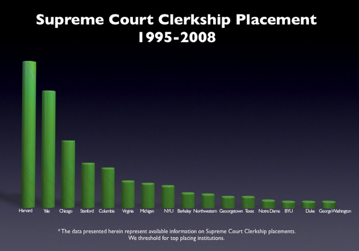
The Clerkship Tournament: Supreme Court Edition [Repost from 6/3]
As part our multipart series on the clerkship tournament, here is a simple bar graph for the top placing law schools in the Supreme Court Clerkship Tourney. It is important to note that we do not threshold for the number of graduates per school. Specifically, we do not just divide by the number graduates per school because we have little theoretic reason to believe that placements linearly scale to differences in size of graduating classes. In other words, given we do not know the proper functional form — we just offer the raw data. For those interested in other posts, please click here for the law clerks tag.
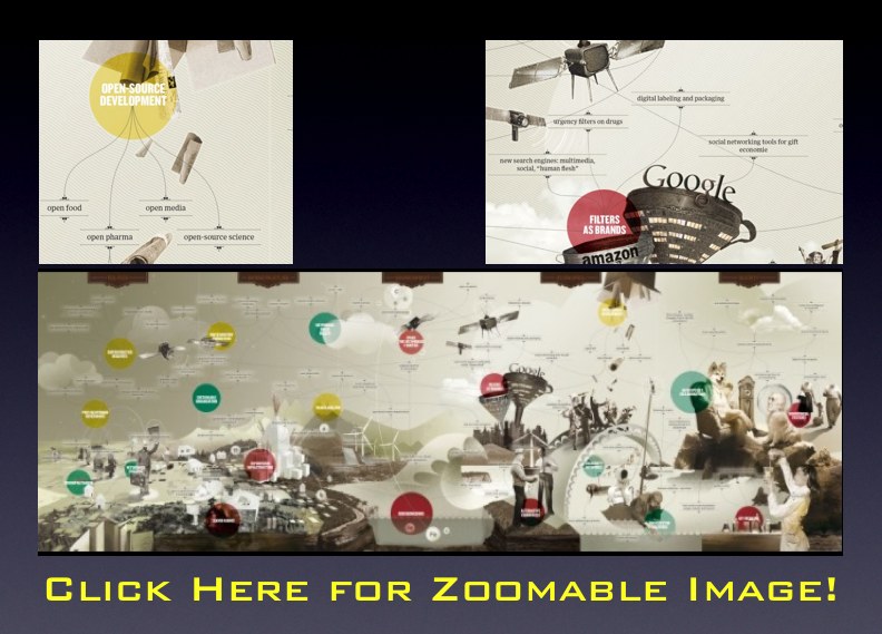
The Map of the Future [From Densitydesign.org]
 As we mentioned in previous posts, Seadragon is a really cool product. Please note load times may vary depending upon your specific machine configuration as well as the strength of your internet connection. For those not familiar with how to operate it please see below. In our view, the Full Screen is best the way to go ….
Who Should Win (probably not who will win) the 2009 Sveriges Riksbank Prize in Economic Sciences in Memory of Alfred Nobel
Benoît Mandelbrot whose classic work on fractals as well as more recent work questioning the Efficient Market Hypothesis offers a lasting contribution to positive economic theory. While the committee is likely considering Eugene Fama and/or Kenneth French (of Fama-French fame), we believe they should instead consider Mandelbrot (or at a minimum split the award between Fama, French & Mandelbrot).
Robert Axelrod whose work on the evolution of cooperation is among the most cited work in all of the social sciences. Iterated Prisoners Dilemma as well as concepts such Tit for Tat are part of the cannon of almost all introductory courses in game theory.
Robert Shiller for his contributions to behavioral finance including his work challenging the Efficient Market Hypothesis. Of course, Shiller is also well known for his work on the real estate market with Karl Case (including the Case-Shiller Index). This also represents important work worthy of recognition.
Elinor Ostrom for her work on public choice theory, common pool resources and collective action. Her work has offered a substantial contribution to political economy as well as institutional and environmental economics. {Note: (Ladbrokes places her at 50 to 1)}.
UPDATE: ELINOR OSTROM AND OLIVER WILLIAMSON WIN THE 2009 NOBEL PRIZE {In Our Estimation, this is a Very Appropriate Decision }
Programming Dynamic Models in Python
 In this series of tutorials, we are going to focus on the theory and implementation of transmission models in some kind of population.
In epidemiology, it is common to model the transmission of a pathogen from one person to another. In the social sciences and law, we may be interested in thinking about the way in which individuals influence each other’s opinions, ideology and actions.
These two examples are different, but in many ways analogous: it is not difficult to imagine the influence that one individual has on another as being similar to the infectivity of a virus in the sense that both have the ability to change the state of an individual. One may go from being susceptible to being infected, or from unconvinced to convinced.
Additionally, social networks have become an important area of study for epidemiological modelers. We can imagine that the nature of the network is different than the ones we think about in the social sciences: when studying outbreaks of a sexually transmitted disease, one doesn’t care all that much about the friendship networks of the people involved, while this would be very important for understanding the impact of social influence on depression and anxiety.
As someone who spends a lot of time working in the space where epidemiology and sociology overlap, I end up thinking a lot about these models – and their potential application to new and different problems and am really excited to share them with a broader audience here. In this first tutorial, I’m going to introduce a simple Susceptible-Infected-Recovered (SIR) model from infectious disease epidemiology and show a simple, Pythonic implementation of it. We’ll work through the process of writing and optimizing this kind of model in Python and, in the final tutorials, will cover how to include a social network in the simulation model.
In order to use the example below, all you need to have installed is a current version of Python (2.4+ is probably best) and the excellent Python plotting package Matplotlib in order to view output. If you don’t have Matplotlib and don’t want to go and install it (although I guarantee you won’t regret it), just comment out import for Pylab and any lines related to plotting.
Model Assumptions
1. State Space / Markov Model
Before getting into the mechanics of the model, let’s talk about the theory and assumptions behind the model as it is implemented here:
The SIR model is an example of a ‘state space‘ model, and the version we’ll be talking about here is a discrete time, stochastic implementation that has the Markov property, which is to say that its state at time t+1 is only conditional on the parameters of the model and its state at time t.
For the uninitiated, in a state-space model, we imagine that each individual in the system can only be in one state at a time and transitions from state to state as a function of the model parameters, i.e., the infectivity of the pathogen or idea and the rate of recovery from infection…and the other states of the system. In other words, the system has endogenous dynamics. This is what makes it both interesting and in some ways difficult to work with.
In the SIR model, we assume that each infectious individual infects each susceptible individual at rate beta. So, if beta = .5, there is a 50% chance that each susceptible individual will be infected by an exposure to an infectious individual. For this reason, as the number of infected individuals in the system grows, the rate at which the remaining susceptible individuals is infected also grows until the pool of susceptible individuals is depleted and the epidemic dies out.
The other parameter we care about is gamma, or the rate of recovery. If gamma is also equal to .5, we assume that the average individual has a 50% chance of recovering on a given day, and the average duration of infectiousness will be 1/gamma, or 2 days.
We refer to the ratio beta/gamma as the basic reproductive ratio, or Ro (‘R naught’). When this number is less than one, we typically expect outbreaks to die out quickly. When this quantity is greater than one, we expect that the epidemic will grow and potentially saturate the whole population.
2. Homogeneous Mixing:
We’re assuming a world in which everyone has simultaneous contact with everyone else. In other words, we’re thinking of a totally connected social network. If you’re a regular reader of this blog, a social network enthusiast, or in some other way a thinking person, this assumption probably seems unreasonable. It turns out, however, that for many diseases, this assumption of homogeneous or ‘mass-action’ mixing, which was actually originally borrowed from chemistry, turns out to be a reasonable approximation.
For instance, if we are trying to approximate the transmission dynamics of a very infectious pathogen like measles in a city or town, we can usually overlook social network effects at this scale and obtain a very good fit to the data. This is because even very weak contacts can transmit measles, so that friendships and other types of close contacts are not good predictors of risk. Instead, we we are better off looking at a higher level of organization – the pattern of connection between towns and cities to understand outbreaks. In a social context, something like panic may be thought of as being super-infectious (for a really interesting study about the potential relationship between social panic and flu dynamics, see this paper by Josh Epstein).
This is, however, a generally problematic assumption for most problems of social influence, but an understanding of this most basic version of the model is necessary to move on to more complicated contact patterns.
3. Exponentially distributed infectious periods:
In the most basic implementation of the SIR model, we assume that each infectious individual has some probability of recovering on every step. If our model steps forwards in days and individuals have a .5 probability of recovery on each day, we should expect that the time to recovery follows an exponential distribution. This means that most people will be pretty close to the mean, but some will take a relatively long time to recover. This is accurate for a lot of cases, but definitely not for all. In some diseases, recovery times may be lognormal, power-law or bimodally disributed. For social models, the notion of an ‘infectious period’ may not make a tremendous amount of sense at all. But it allows for a very simple and transparent implementation, so we’ll use it here.
CLICK THROUGH TO SEE THE IMPLEMENTATION and RELEVANT PYTHON CODE!

