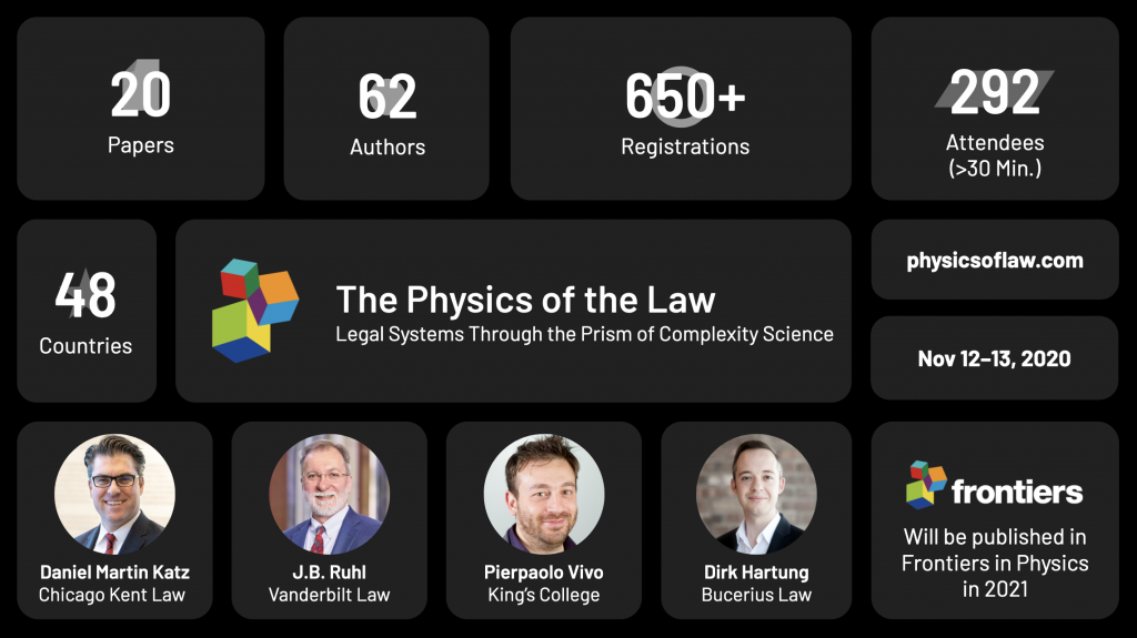
Thanks to everyone who attended The Physics of Law Virtual Conference earlier this month. Overall, we had 292+ Attendees from 48 Countries watch the presentation of 20 Academic Papers by 62 Authors. We saw a wide range of methods from Physics, Computer Science and Applied Mathematics devoted to the exploration of legal systems and their outputs.
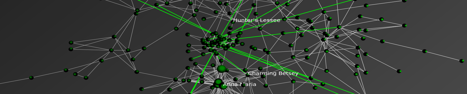
Methodological approaches included Agent Based Modeling, Game Theory and other Formal Modeling, Dynamics of Acyclic Digraphs, Knowledge Graphs, Entropy of Legal Systems, Temporal Modeling of MultiGraphs, Information Diffusion, etc.
NLP Methods on display included traditional approaches such as TF-IDF, n-grams, entity identification and other metadata extraction as well as more advanced methods such as Bert, Word2Vec, GloVe, etc.
Methods were then applied to topics including Attorney Advocacy Networks, Statutory Outputs from Legislatures, various bodies of Regulations, Contracts, Patents, Shell Corporations, Common Law Systems, Legal Scholarship and Legal Rules ∩ Financial Systems.
If you have an eligible paper – it is not too late to submit – papers are due in January. After undergoing the Peer Review process — Look for the Final Papers to be published in Frontiers in Physics in 2021.