
Tag: social epidemiology
Law Professoriate Poster for Conference on Empirical Legal Studies (CELS 2009 @ USC)

 As we mentioned in previous posts, Seadragon is a really cool product. Please note load times may vary depending upon your specific machine configuration as well as the strength of your internet connection. For those not familiar with how to operate it please see below. In our view, the Full Screen is best the way to go ….
Programming Dynamic Models in Python-Part 3: Outbreak on a Network
In this post, we will continue building on the basic models we discussed in the first and second tutorials. If you haven’t had a chance to take a look at them yet, definitely go back and at least skim them, since the ideas and code there form the backbone of what we’ll be doing here.
In this tutorial, we will build a model that can simulate outbreaks of disease on a small-world network (although the code can support arbitrary networks). This tutorial represents a shift away from both:
a) the mass-action mixing of the first two and and
b) the assumption of social homogeneity across individuals that allowed us to take some shortcuts to simplify model code and speed execution. Put another way, we’re moving more in the direction of individual-based modeling.
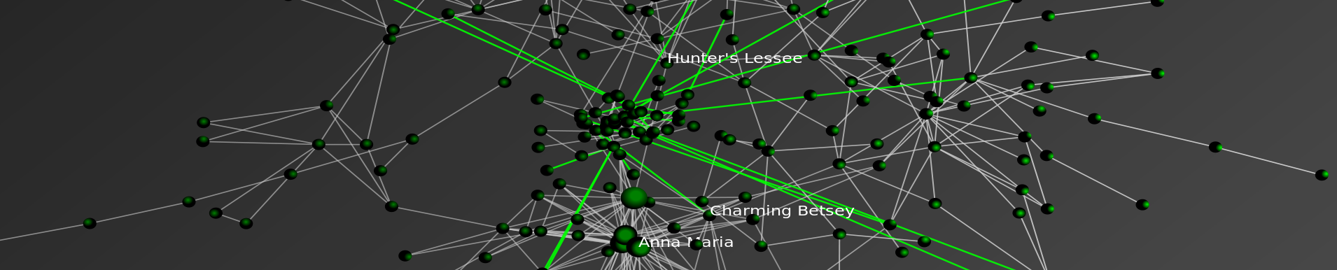
When we’re done, your model should be producing plots that look like this:

Red nodes are individuals who have been infected before the end of the run, blue nodes are never-infected individuals and green ones are the index cases who are infectious at the beginning of the run.
And your model will be putting out interesting and unpredictable results such as these:

In order to do this one, though, you’re going to need to download and install have igraph for Python on your system.
Individual-Based Networks
It is important to make the subtle distinction between individual and agent based models very clear here. Although the terms are often used interchangeably, referring to our nodes, who have no agency, per se, but are instead fairly static receivers and diffusers of infection, as agents, seems like overreaching. Were they to exhibit some kind of adaptive behavior, i.e., avoiding infectious agents or removing themselves from the population during the infective period, they then become more agent-like.
This is not to under- or over-emphasize the importance or utility of either approach, but just to keep the distinction in mind to avoid the “when all you have is a hammer, everything looks like a nail” problem.
In short, adaptive agents are great, but they’re overkill if you don’t need them for your specific problem.
Small World Networks
The guiding idea behind small-world networks is that they capture some of the structure seen in more realistic contact networks: most contacts are regular in the sense that they are fairly predicable, but there are some contacts that span tightly clustered social groups and bring them together.
In the basic small-world model, an individual is connected to some (small, typically <=8) number of his or her immediate neighbors. Some fraction of these network connections are then randomly re-wired, so that some individuals who were previously distant in network terms – i.e., connected by a large number of jumps – are now adjacent to each other. This also has the effect of shortening the distance between their neighbors and individuals on the other side of the graph. Another way of putting this is that we have shortened the average path length and increased the average reachability of all nodes.
These random connections are sometimes referred to as “weak ties”, as there are fewer of these ties that bridge clusters than there are within clusters. When these networks are considered from a sociological perspective, we often expect to find that the relationship represented by a weak tie is one in which the actors on either end have less in common with each other than they do with their ‘closer’ network neighbors.
Random networks also have the property of having short average path lengths, but they lack the clustering that gives the small-world model that pleasant smell of quasi-realism that makes them an interesting but largely tractable, testing ground for theories about the impact of social structure on dynamic processes.
Installation and Implementation Issues
If you have all the pre-requisites installed on your system, you should be able to just copy and paste this code into a new file and run it with your friendly, local Python interpreter. When you run the model, you should first see a plot of the network, and when you close this, you should see a plot of the number of infections as a function of time shortly thereafter.
Aside from the addition of the network, the major conceptual difference is that the model operates on discrete individuals instead of a homogeneous population of agents. In this case, the only heterogeneity is in the number and identity of each individual’s contacts, but there’s no reason we can’t (and many do) incorporate more heterogeneity (biological, etc.) into a very similar model framework.
With Python, this change in orientation to homogeneous nodes to discrete individuals seems almost trivial, but in other languages it can be somewhat painful. For instance, in C/++, a similar implementation would involve defining a struct with fields for recovery time and individual ID, and defining a custom comparison operator for these structs. Although this is admittedly not a super-high bar to pass, it adds enough complexity that it can scare off novices and frustrate more experienced modelers.
Perhaps more importantly, it often has the effect of convincing programmers that a more heavily object-oriented approach is the way to go, so that each individual is a discrete object. When our individuals are as inert as they are in this model, this ends up being a waste of resources and makes for significantly more cluttered code. The end result can often be a model written in a language that is ostensibly faster than Python, such as C++ or Java, that runs slower than a saner (and more readable) Python implementation.
For those of you who are playing along at home, here are some things to think about and try with this model:
- Change the kind of network topology the model uses (you can find all of the different networks available in igraph here).
- Incorporate another level of agent heterogeneity: Allow agents to have differing levels of infectivity (Easier); Give agents different recovery time distributions (Harder, but not super difficult).
- Make two network models – you can think of them as separate towns – and allow them to weakly influence each other’s outbreaks. (Try to use the object-oriented framework here with minimal changes to the basic model.)
That’s it for tutorial #3, (other than reviewing the comment code which is below) but definitely check back for more on network models!
In future posts, we’ll be thinking about more dynamic networks (i.e., ones where the links can change over time), agents with a little more agency, and tools for generating dynamic visualizations (i.e., movies!) of stochastic processes on networks.
That really covers the bulk of the major conceptual issues. Now let’s work through the implementation.
Click Below to Review the Implementation and Commented Code!
Continue reading “Programming Dynamic Models in Python-Part 3: Outbreak on a Network”

Programming Dynamic Models in Python: Coding Efficient Dynamic Models
 In the next few tutorials, we’re going to transition to exploring how to model dynamics on a network.
The first tutorial was a bit of a blockbuster length-wise because there was a lot of ground to cover to get the basic model up and running. Moving forward, we’ll be able to go a bit more incrementally, adding elements to the basic model as we go. If you don’t feel comfortable with the original, go back and take a look at it and make sure that it makes sense to you before moving on.
We’re first going to deal with some of the efficiency issues in the first model. After this, we’ll make some basic changes to the architecture of the SIR program that makes it more amenable to contact patterns on a social network.
Finally, we’ll show you how to how to take the output of your epidemic model and generate animations like this one:
Blue nodes are exposed but uninfected, red nodes are infectious, and yellow ones have recovered.
The movie is a bit of a carrot to get you through the less flashy, but, I promise, important and actually interesting nuts and bolts of putting these kinds of models together.
This tutorial is going to cover the last two big things that we need to tackle before we get to the model of an outbreak on a network. So, here we go!
New Concepts
1. Arbitrarily Distributed Infectious Periods
First, we’re going to deal with the duration of the infectious period. The assumption of an exponentially distributed infectious period is unnecessarily restrictive for a general model of diffusion, and the way the original code goes about recovering individuals – drawing a random number on every step for every infectious individual – should strike you as both inelegant and computationally inefficient, particularly when the rate of recovery is slow and there are many infectious individuals.
In order to deal with this, we’re going to introduce two new tools. The first is the scipy.stats toolkit and the second is a neat (and very easy to use) data structure called a heap.
A heap is in very many ways what it sounds like: imagine a pile of trash in a landfill; the tires and rusting washing machines are on the bottom, while the pop cans and grocery store receipts are closer to the top.
As a programming tool, a heap is useful because it always keeps the smallest (or largest, depending on your preference) item at the top of the list. It also allows for linear-time insertion and removal of objects. This means that the time it takes to execute an action grows proportionally to the size of the list, so if it has N items, it takes N*C steps (where C is a constant) to process the list, and if it has 2*N items, it takes 2*N*C steps. Other ways of sorting could take N^2 or worse steps to do the same.
In our outbreak model, the top item on the heap is always going to be the time at which the next individual recovers. By doing this, we can avoid the loop in the first tutorial (and replicated in one implementation here) that checks whether each infectious individual is going to recover on each step.
Looping over everyone is the most intuitive way to check if they’re going to recover, but it’s very inefficient, especially when infectious periods are long and the population is large. It’s also problematic from a theoretical perspective, because it chains us to exponentially distributed recovery periods.
Exponentially distributed infectious periods make analytic sense for a deterministic model, but your disease or *insert diffusible here* may have a constant or normally distributed ‘infectious’ period.
By using a heap-based implementation, as you will see, we can use arbitrary recovery periods, and Python’s implementation of the heap is very straightforward – just a small twist on the usual list using the heapq module.
2. Object Oriented Programming
One of Python’s strengths is that it supports a style of programming that mixes the best of object-oriented programming (OOP) and procedural or imperative programming.
We won’t go too deep into the details of OOP here, but the real strength of OOP implementations are that they allow code to be easily re-used in other programs (Python’s all-powerful ‘import‘ statement really makes this true) and also forces some structure on what functions have access to what variables, etc.
Click Below to Review the Implementation and Commented Code!
Continue reading “Programming Dynamic Models in Python: Coding Efficient Dynamic Models”
Programming Dynamic Models in Python
 In this series of tutorials, we are going to focus on the theory and implementation of transmission models in some kind of population.
In epidemiology, it is common to model the transmission of a pathogen from one person to another. In the social sciences and law, we may be interested in thinking about the way in which individuals influence each other’s opinions, ideology and actions.
These two examples are different, but in many ways analogous: it is not difficult to imagine the influence that one individual has on another as being similar to the infectivity of a virus in the sense that both have the ability to change the state of an individual. One may go from being susceptible to being infected, or from unconvinced to convinced.
Additionally, social networks have become an important area of study for epidemiological modelers. We can imagine that the nature of the network is different than the ones we think about in the social sciences: when studying outbreaks of a sexually transmitted disease, one doesn’t care all that much about the friendship networks of the people involved, while this would be very important for understanding the impact of social influence on depression and anxiety.
As someone who spends a lot of time working in the space where epidemiology and sociology overlap, I end up thinking a lot about these models – and their potential application to new and different problems and am really excited to share them with a broader audience here. In this first tutorial, I’m going to introduce a simple Susceptible-Infected-Recovered (SIR) model from infectious disease epidemiology and show a simple, Pythonic implementation of it. We’ll work through the process of writing and optimizing this kind of model in Python and, in the final tutorials, will cover how to include a social network in the simulation model.
In order to use the example below, all you need to have installed is a current version of Python (2.4+ is probably best) and the excellent Python plotting package Matplotlib in order to view output. If you don’t have Matplotlib and don’t want to go and install it (although I guarantee you won’t regret it), just comment out import for Pylab and any lines related to plotting.
Model Assumptions
1. State Space / Markov Model
Before getting into the mechanics of the model, let’s talk about the theory and assumptions behind the model as it is implemented here:
The SIR model is an example of a ‘state space‘ model, and the version we’ll be talking about here is a discrete time, stochastic implementation that has the Markov property, which is to say that its state at time t+1 is only conditional on the parameters of the model and its state at time t.

For the uninitiated, in a state-space model, we imagine that each individual in the system can only be in one state at a time and transitions from state to state as a function of the model parameters, i.e., the infectivity of the pathogen or idea and the rate of recovery from infection…and the other states of the system. In other words, the system has endogenous dynamics. This is what makes it both interesting and in some ways difficult to work with.
In the SIR model, we assume that each infectious individual infects each susceptible individual at rate beta. So, if beta = .5, there is a 50% chance that each susceptible individual will be infected by an exposure to an infectious individual. For this reason, as the number of infected individuals in the system grows, the rate at which the remaining susceptible individuals is infected also grows until the pool of susceptible individuals is depleted and the epidemic dies out.
The other parameter we care about is gamma, or the rate of recovery. If gamma is also equal to .5, we assume that the average individual has a 50% chance of recovering on a given day, and the average duration of infectiousness will be 1/gamma, or 2 days.
We refer to the ratio beta/gamma as the basic reproductive ratio, or Ro (‘R naught’). When this number is less than one, we typically expect outbreaks to die out quickly. When this quantity is greater than one, we expect that the epidemic will grow and potentially saturate the whole population.
2. Homogeneous Mixing:
We’re assuming a world in which everyone has simultaneous contact with everyone else. In other words, we’re thinking of a totally connected social network. If you’re a regular reader of this blog, a social network enthusiast, or in some other way a thinking person, this assumption probably seems unreasonable. It turns out, however, that for many diseases, this assumption of homogeneous or ‘mass-action’ mixing, which was actually originally borrowed from chemistry, turns out to be a reasonable approximation.
For instance, if we are trying to approximate the transmission dynamics of a very infectious pathogen like measles in a city or town, we can usually overlook social network effects at this scale and obtain a very good fit to the data. This is because even very weak contacts can transmit measles, so that friendships and other types of close contacts are not good predictors of risk. Instead, we we are better off looking at a higher level of organization – the pattern of connection between towns and cities to understand outbreaks. In a social context, something like panic may be thought of as being super-infectious (for a really interesting study about the potential relationship between social panic and flu dynamics, see this paper by Josh Epstein).
This is, however, a generally problematic assumption for most problems of social influence, but an understanding of this most basic version of the model is necessary to move on to more complicated contact patterns.
3. Exponentially distributed infectious periods:
In the most basic implementation of the SIR model, we assume that each infectious individual has some probability of recovering on every step. If our model steps forwards in days and individuals have a .5 probability of recovery on each day, we should expect that the time to recovery follows an exponential distribution. This means that most people will be pretty close to the mean, but some will take a relatively long time to recover. This is accurate for a lot of cases, but definitely not for all. In some diseases, recovery times may be lognormal, power-law or bimodally disributed. For social models, the notion of an ‘infectious period’ may not make a tremendous amount of sense at all. But it allows for a very simple and transparent implementation, so we’ll use it here.
CLICK THROUGH TO SEE THE IMPLEMENTATION and RELEVANT PYTHON CODE!
Christakis and Fowler in Wired Magazine

Today marks the official release of Connected: The Surprising Power of Our Social Networks and How They Shape Our Lives by Nicholas A. Christakis & James H. Fowler. There has been some really good publicity for the book including the cover story in last Sunday’s New York Times Magazine. However, given the crisp visualizations — my favorite is the above article from Wired Magazine. Click on the visual above to read the article!
Positive Legal Theory and a Model of Intellectual Diffusion on the American Legal Academy [Repost from 4/22]
 For the third installment of posts related to Reproduction of Hierarchy? A Social Network Analysis of the American Law Professoriate, we offer a Netlogo simulation of intellectual diffusion on the network we previously visualized. As noted in prior posts, we are interested legal socialization and its role in considering the spread of particular intellectual or doctrinal paradigms. This model captures a discrete run of the social epidemiological model we offer in the paper. As we noted within the paper, this represents a first cut on the question—where we favor parsimony over complexity. In reality, there obviously exist far more dynamics than we engage herein. The purpose of this exercise is simply to begin to engage the question. In our estimation, a positive theory of law should engage the sociology of the academy — a group who collectively socialize nearly every lawyer and judge in the United States. In the paper and in the model documentation, we offer some possible model extensions which could be considered in future scholarship.
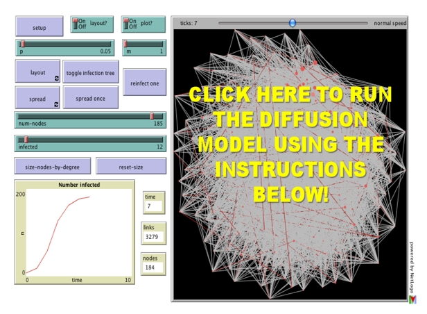
Once you click through to the model, here is how it works:
(1) Click the Setup Button in the Upper Left Corner. This will Display the Network in the Circular Layout.
(2) Click the Layout Button. Depending upon the speed of your machine this may take up to 30 seconds. Stop the Layout Button by Re-Clicking the Button.
(3) Click the Size Nodes by Degree Button. You Will Notice the Fairly Central Node Colored in Red. This is School #12 Northwestern University Law School. Observe how we have set the default infected school as #12 Northwestern (Hat Tip to Uri Wilensky). A Full List of School Number is available at the bottom of the page when you click through.
(4) Now, we are ready to begin. Click the Spread Once Button. The idea then reaches its neighbors with probability p (set as a default at .05). You can click the Toggle Infection Tree button (at any point) to observe the discrete paths traversed by the idea.
(5) Click the Spread Once Button, again and again. Notice the plot tracking the time on the x axisand the number of institution infected on the y axis. This is an estimate of the diffusion curve for the institution.
(6) To restart the simulation, click the Reinfect One button. Prior to hitting this button, slide theInfected Slider to any Law School you would like to observe. Also, feel free to adjust the p slider to increase or decrease the infectiousness of the idea.
Please comment if you have any difficulty or questions. Note you must have Java 1.4.1 + installed on your computer. The Information Technology professionals at many institutions will have already installed this on your machine but if not you will need to download it. We hope you enjoy!
State Level Obesity Trends from the CDC Website

It has been light blogging while we finish some projects here in Ann Arbor. In the meantime, here is an interesting visual offered by CDC website. Also, check out an important paper in this vein by Nicholas Christakis & James Fowler entitled The Spread of Obesity in a Large Social Network Over 32 Years (Click to the Left to Link to the Original Movie). Anyway, more to come later in the week…
The S.I.R. Model — A Simple Model With Applications to Swine Flu, etc.

Last week we offered a model of intellectual diffusion built upon a standard fare social epidemiology model. Given recent events within the United States, Mexico and potentially worldwide, we thought it would be worthwhile to highlight the classic S.I.R. (Susceptible, Infected, Recovered) model. Netlogo offers a user friendly version of the model. Using this platform, we hope the exploration of the dynamics of S.I.R. might prove illuminating.
First, various hosts have different levels of interactions (work, home, transit, etc.) and so this network approach represents a blunt measure. To start the model at the default parameters, push the SETUP Button and then the GO Button. As the model runs, the plot tracks the Susceptible, Infected, Recovered. The model contains a variety of “sliders.” The model can be rerun at lots of combinations of parameter levels. Those “sliders” fall into several categories: Network Attributes, Virus Attributes, Node Attributes. The full documentation is available here.
With respect to the swine flu, one important parameter is the delay between when an individual becomes infectious and when that individual is likely to become symptomatic. This parameter can be tuned in the simulation above using VIRUS-CHECK-FREQUENCY slider. From the documentation… “Infected nodes are not immediately aware that they are infected. Only every so often (determined by the VIRUS-CHECK-FREQUENCY slider) do the nodes check whether they are infected by a virus.”
An additional parameter worthy of consideration is the VIRUS-SPREAD-CHANCE. Consider this slider as a rough measure of the underlying infectiousness of the virus in question.
It is important to note the above simulation is an incredible simplification of the world faced by public health officials. Additionally, this version of the model was designed to consider the spread of disease on a computer network. Notwithstanding these limitations, we thought it useful to highlight a computational approach to this important matter of public concern.
The Revolution Will Not Be Televised — But Will it Come from HLS or YLS ? A Social Network Analysis of the Legal Academy (Part IV)

This is the final installment of posts related to Reproduction of Hierarchy? A Social Network Analysis of the American Law Professoriate. Thanks for your emails.
Here is the plot we provide within the paper. As a general proposition, we believe this represents an upper bound measure for the intellectual reach of an agenda offered by a given institution. With respect to our version of the Reed Frost Epidemiological Model, we use the p parameter to model “idea infectiousness.” When p = 1 every institution “contacted” by the idea is infected with the idea. When p = 0 no institution “contacted” by the idea is infected. In this version, we use the programming language python to run the model 500 times per institution. The above plot represents an estimate of the “diffusion curve” for each of the 184 institutions in our model. Building off central limit type properties, this leaves a far better estimate of reach than is offered in the single model run from the previous Netlogo GUI.
A cursory review of the above plot demonstrates, we are far from the land of linearity. Namely, a large number of institutions are able to reach much of the graph with very small changes in the value of p.
In the Structure of Scientific Revolutions, Kuhn quotes from Max Planck: “a new scientific truth does not triumph by convincing its opponents and making them see the light, but rather because its opponents eventually die, and a new generation grows up that is familiar with it.” Following Planck, we believe retirement is indeed be an important mechanism. However, we also argue the nature of the p parameter is a relevant consideration. In fact, unpacking various dimensions of p is the key to the broader model. Specifically, what are the properties of an idea that generate its infectiousness? Of course, we might like to believe infectiousness is related to a class of normatively attractive properties such as promoting efficiency or justice. However, it is not clear that this follows.
We took no pass on the question of whether some institutions would be better or worse at producing ideas with greater or lesser values of p. The motivated question for this post considers whether, in general, the institutions which are top producers of law professors are (1) leaders in innovation, (2) subsequent ratifiers of a newly established paradigm or (3) defenders of the status quo. In a deep sense, we are asking how to reasonably model decision making by the heterogeneous agents located at such institutions. Do institutions reward or punish intellectual risk-taking, search, etc.?
While this is an empirical question beyond the scope of this post, it worth asking because it partially informs the micro-dynamics plausibly responsible for generating the spread of new intellectual paradigms.
Model of Intellectual Diffusion Upon the American Legal Academy
 For the third installment of posts related to Reproduction of Hierarchy? A Social Network Analysis of the American Law Professoriate, we offer a Netlogo simulation of intellectual diffusion on the network we previously visualized. As noted in prior posts, we are interested legal socialization and its role in considering the spread of particular intellectual or doctrinal paradigms. This model captures a discrete run of the social epidemiological model we offer in the paper. As we noted within the paper, this represents a first cut on the question—where we favor parsimony over complexity. In the paper and in the model documentation, we offer some possible model extensions which could be considered in future scholarship.
Once you click through to the model, here is how it works:
(1) Click the Setup Button in the Upper Left Corner. This will Display the Network in the Circular Layout.
(2) Click the Layout Button. Depending upon the speed of your machine this may take up to 30 seconds. Stop the Layout Button by Re-Clicking the Button.
(3) Click the Size Nodes by Degree Button. You Will Notice the Fairly Central Node Colored in Red. This is School #12 Northwestern University Law School. Observe how we have set the default infected school as #12 Northwestern (Hat Tip to Uri Wilensky). A Full List of School Number is available at the bottom of the page when you click through.
(4) Now, we are ready to begin. Click the Spread Once Button. The idea then reaches its neighbors with probability p (set as a default at .05). You can click the Toggle Infection Tree button (at any point) to observe the discrete paths traversed by the idea.
(5) Click the Spread Once Button, again and again. Notice the plot tracking the time on the x axis and the number of institution infected on the y axis. This is an estimate of the diffusion curve for the institution.
(6) To restart the simulation, click the Reinfect One button. Prior to hitting this button, slide the Infected Slider to any Law School you would like to observe. Also, feel free to adjust the p slider to increase or decrease the infectiousness of the idea.
Please comment if you have any difficulty or questions. Note you must have Java 1.4.1 + installed on your computer. The Information Technology professionals at many institutions will have already installed this on your machine but if not you will need to download it. We hope you enjoy!